This lab is due at 11:59pm on 09/17/2014.
Please start at the beginning of the lab and work your way through, working and talking over Python's behavior in the conceptual questions with your classmates nearby. These questions are designed to help you experiment with the concepts on the Python interpreter or Python Tutor. They are good tests for your understanding.
When you are done with lab, you have to submit Questions 3, 4, 6, and 8 to receive credit for this lab. Questions 5, 9, and 10 are marked with an asterisk and considered extra practice. It is recommended that you complete these problems on your own time.
By the end of this lab, you should have submitted the
lab03assignment using the commandsubmit lab03. You can check if we received your submission by runningglookup -t.
The starter file lab03.py contains all of the questions you must submit. In addition, the lab03_extra.py file contains all of the extra practice questions. Click here to see more complete submission instructions.
Last week in lab, we looked at some error messages that Python interpreter would give. This time, we will look at output from the doctest module. If you are comfortable with using doctests and reading doctest output, please feel free to skip this section.
Recall that to run doctests on a file (can be a text file as well!), one would enter this command to the shell:
python3 -m doctest path/to/fileIt's important to understand that you must locate the specific file
by name, unlike the submit command from the class account, which
takes in the assignment name (not the file name) as input.
Just to see the difference, try:
python3 -m doctest lab03Unless you have a file named lab03 without an extension, Python
will raise an exception that looks like:
FileNotFoundError: [Errno 2] No such file or directory: 'lab03'Side note: extensions are not a separate part of the file name. You can have file names like
lab03.py.old, orlab03. Python will just assume that it can treat any file ending with.pyas Python code.
Now try running doctests with lab03.py, the actual name of
the file you just downloaded:
python3 -m doctest lab03.pyThe final part of the output (the summary) looks like:
9 items had failures:
1 of   1 in lab03.f1
1 of   1 in lab03.f2
1 of   1 in lab03.f3
1 of   1 in lab03.f4
1 of   1 in lab03.f5
2 of   2 in lab03.hailstone
3 of   3 in lab03.lambda_curry2
4 of   4 in lab03.mul_by_num
2 of   2 in lab03.sum
***Test Failed*** 16 failures.
Each item refers to a function or class that can be accessed
from the Python file. Some functions may not have doctests, in
which case, the doctest will say x items had no tests. Here,
we can see that lab03.sum has 2 tests. What are they?
>>> sum(1)
1
>>> sum(5)
15
We can thus see that the two tests are the two expressions fed
into the interactive console (>>>) followed by the expected
output.
Let's examine the failure output of a particular test:
**********************************************************************
File "/path/to/lab03.py", line 71, in lab03.sum
Failed example:
sum(5)  # 1 + 2 + 3 + 4 + 5
Expected:
15
Got nothing
**********************************************************************
On the first line, you see the file name, line number, and the particular item from the module. You can compare the parts in this output to the test shown above. The expression in the interactive console is known as the "example" here. The expected output is what you place inside your program next to your test. Finally, Python will actually run your code and compare that result with what you expect. If there are differences, Python will display them, or else Python will say 'ok'.
To see all the tests that are run, even the successful ones, remember that you can enter the following to your terminal:
python3 -m doctest -v lab03.pyRemember, passing all the doctests does not guarantee that your code is completely correct. Nevertheless, they are a great way to catch any bugs you may have overlooked in your code.
Great! Now you should be more familiar with the output from doctest, which should make your debugging more effective. Always feel free to supplement our tests with your own. Writing tests for a problem can even help you understand the problem better!
Now we'll see where environment diagrams come in really handy: When dealing with lambda expressions in addition to other higher-order functions.
Lambda expressions are one-line functions that specify two things: the parameters and the return value.
lambda <parameters>: <return value>One difference between using the def keyword and lambda
expressions is that def is a statement, while lambda is an
expression. Evaluating a def statement will have a side effect;
namely, it creates a new function binding in the current environment.
On the other hand, evaluating a lambda expression will not change the
environment unless we do something with this expression. For instance,
we could assign it to a variable or pass it in as a function argument.
>>> a = lambda: 5
>>> a()
______5
>>> a(5)
______TypeError: <lambda>() takes 0 positional arguments but 1 was given
>>> a()()
______TypeError: 'int' object is not callable
>>> b = lambda: lambda x: 3
>>> b()(15)
______3
>>> c = lambda x, y: x + y
>>> c(4, 5)
______9
>>> d = lambda x: c(a(), b()(x))
>>> d(2)
______8
>>> b = lambda: lambda x: x
>>> d(2)
______7
>>> e = lambda x: lambda y: x * y
>>> e(3)
______<function ...>
>>> e(3)(3)
______9
>>> f = e(2)
>>> f(5)
______10
>>> f(6)
______12
>>> g = lambda: print(1) # When is the body of this function run?
______# Nothing gets printed by the interpreter
>>> h = g()
______1
>>> print(h)
______NoneTry drawing environment diagrams for the following code and predicting what Python will output:
>>> # Part 1
>>> a = lambda x : x * 2 + 1
>>> def b(x):
...     return x * y
...
>>> y = 3
>>> b(y)
______9
>>> def c(x):
...     y = a(x)
...     return b(x) + a(x+y)
...
>>> c(y)
______30
>>> # Part 2: This one is pretty tough. A carefully drawn environment
>>> # diagram will be really useful.
>>> g = lambda x: x + 3
>>> def wow(f):
...     def boom(g):
...       return f(g)
...     return boom
...
>>> f = wow(g)
>>> f(2)
______5
>>> g = lambda x: x * x
>>> f(3)
______6g = lambda x: x * x doesn't change what f(3) does!
For each of the following expressions, write functions f1, f2,
f3, and f4 such that the evaluation of each expression
succeeds, without causing an error. Be sure to use lambdas in your
function definition instead of nested def statements. Each function
should have a one line solution.
def f1():
    """
    >>> f1()
    3
    """
    "*** YOUR CODE HERE ***"
    return 3
def f2():
    """
    >>> f2()()
    3
    """
    "*** YOUR CODE HERE ***"
    return lambda: 3
def f3():
    """
    >>> f3()(3)
    3
    """
    "*** YOUR CODE HERE ***"
    return lambda x: x
def f4():
    """
    >>> f4()()(3)()
    3
    """
    "*** YOUR CODE HERE ***"
return lambda: lambda x: lambda: xWe can transform multiple-argument functions into a chain of single-argument, higher order functions by taking advantage of lambda expressions. This is useful when dealing with functions that take only single-argument functions. We will see some examples of these later on.
Write a function lambda_curry2 that will curry any two argument
function using lambdas. See the doctest if you're not sure what this
means.
def lambda_curry2(func):
    """
    Returns a Curried version of a two argument function func.
    >>> from operator import add
    >>> x = lambda_curry2(add)
    >>> y = x(3)
    >>> y(5)
    8
    """
    "*** YOUR CODE HERE ***"
    return ______
return lambda arg1: lambda arg2: func(arg1, arg2)Fill in the blanks as to what Python would do here. Please try this problem first with an environment diagram, and then again without an environment diagram.
>>> def troy():
...     abed = 0
...     while abed < 10:
...         britta = lambda: abed
...         abed += 1
...     abed = 20
...     return britta
...
>>> jeff = troy()
>>> shirley = lambda : jeff
>>> pierce = shirley()
>>> pierce()
______20A recursive function is a function that calls itself in its body, either directly or indirectly. Recursive functions have two important components:
Let's look at the canonical example, factorial:
def factorial(n):
    if n == 0:
        return 1
    return n * factorial(n - 1)
We know by its definition that 0! is 1. So we choose n = 0 as our
base case. The recursive step also follows from the definition of
factorial, i.e. n! = n * (n-1)!.
The next few questions in lab will have you writing recursive functions. Here are some general tips:
Write a function sum that takes a single argument n
and computes the sum of all integers between 0 and n inclusive.
Assume n is non-negative.
def sum(n):
    """Computes the sum of all integers between 1 and n, inclusive.
    Assume n is positive.

    >>> sum(1)
    1
    >>> sum(5)  # 1 + 2 + 3 + 4 + 5
    15
    """
    "*** YOUR CODE HERE ***"
    if n == 1:
        return 1
return n + sum(n - 1)The following examples of recursive functions show some examples of common recursion mistakes. Fix them so that they work as intended.
def sum_every_other_number(n):
    """Return the sum of every other natural number
    up to n, inclusive.

    >>> sum_every_other_number(8)
    20
    >>> sum_every_other_number(9)
    25
    """
    if n == 0:
        return 0
    else:
return n + sum_every_other_number(n - 2)Consider what happens when we choose an odd number for n.
sum_every_other_number(3) will return 3 +
sum_every_other_number(1). sum_every_other_number(1) will return
1 + sum_every_other_number(-1). You may see the problem now. Since
we are decreasing n by two at a time, we've completed missed our base
case of n == 0, and we will end up recursing indefinitely. We need to
add another base case to make sure this doesn't happen.
def sum_every_other_number(n):
    if n == 0:
        return 0
    elif n == 1:
        return 1
    else:
        return n + sum_every_other_number(n - 2)
def fibonacci(n):
"""Return the nth fibonacci number.
>>> fibonacci(11)
89
"""
if n == 0:
return 0
elif n == 1:
return 1
else:
fibonacci(n - 1) + fibonacci(n - 2)The result of the recursive calls is not returned.
def fibonacci(n):
    if n == 0:
        return 0
    elif n == 1:
        return 1
    else:
return fibonacci(n - 1) + fibonacci(n - 2)def even_digits(n):
"""Return the percentage of digits in n that are even.
>>> even_digits(23479837) # 3 / 8
0.375
"""
if n == 0:
return num_digits / num_evens
num_digits, num_evens = 0, 0
if n % 2 == 0:
counter += 1
num_evens += 1
return (even_digits(n // 10) + num_evens) / counterWhen we first call even_digits, we set a counter num_digits to 0.
After we increment the counter, when we recurse and call even_digits
again, in the frame of the recursive call we actually create a new
counter variable set to 0. We are therefore not actually accumulating
the number of digits. In order to keep track of information
between recursive calls we need to pass the information as arguments to
functions. Therefore, to solve this problem, we will use a helper
function that we define so that we can choose which arguments to use.
def even_digits(n):
    def helper(n, digits, evens):
        if n == 0:
          return evens / digits
        if n % 2 == 0:
          evens += 1
        return helper(n // 10, digits + 1, even)
    return helper(n, 0, 0)
The helper function has an added bonus of allowing us to choose the best way to represent our output for recursion: having to add numbers to a decimal is messy, so we just figure out the answer by the time we reach the base case and just propagate the answer up. This cool property will actually lead to a more optimized way of doing recursion, as you'll see later in the course.
For the hailstone function from homework 1, you pick a positive
integer n as the start. If n is even, divide it by 2. If n is
odd, multiply it by 3 and add 1. Repeat this process until n is 1.
Write a recursive version of hailstone that prints out the values of
the sequence and returns the number of steps.
def hailstone(n):
    """Print out the hailstone sequence starting at n, and return the
    number of elements in the sequence.

    >>> a = hailstone(10)
    10
    5
    16
    8
    4
    2
    1
    >>> a
    7
    """
    "*** YOUR CODE HERE ***"
    print(n)
    if n == 1:
        return 1
    elif n % 2 == 0:
        return 1 + hailstone(n // 2)
    else: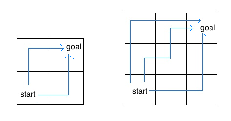
return 1 + hailstone(3 * n + 1)Consider an insect in an M by N grid. The insect starts at the
bottom left corner, (0, 0), and wants to end up at the top right
corner, (M-1, N-1). The insect is only capable of moving right or
up. Write a function paths that takes a grid length and width
and returns the number of different paths the insect can take from the
start to the goal. (There is a closed-form solution to this problem,
but try to answer it procedurally using recursion.)
For example, the 2 by 2 grid has a total of two ways for the insect to move from the start to the goal. For the 3 by 3 grid, the insect has 6 diferent paths (only 3 are shown above).
def paths(m, n):
    """Return the number of paths from one corner of an
    M by N grid to the opposite corner.

    >>> paths(2, 2)
    2
    >>> paths(5, 7)
    210
    >>> paths(117, 1)
    1
    >>> paths(1, 157)
    1
    """
    "*** YOUR CODE HERE ***"
    if m == 1 or n == 1:
        return 1
return paths(m - 1, n) + paths(m, n - 1)The greatest common divisor of two positive integers a and b is the
largest integer which evenly divides both numbers (with no remainder).
Euclid, a Greek mathematician in 300 B.C., realized that the greatest
common divisor of a and b is one of the following:
In other words, if a is greater than b and a is not divisible by
b, then
gcd(a, b) == gcd(b, a % b)Write the gcd function recursively using Euclid's algorithm.
def gcd(a, b):
    """Returns the greatest common divisor of a and b.
    Should be implemented using recursion.

    >>> gcd(34, 19)
    1
    >>> gcd(39, 91)
    13
    >>> gcd(20, 30)
    10
    >>> gcd(40, 40)
    40
    """
    "*** YOUR CODE HERE ***"
    a, b = max(a, b), min(a, b)
    if a % b == 0:
        return b
    else:
        return gcd(b, a % b)

# Iterative solution, if you're curious
def gcd_iter(a, b):
    """Returns the greatest common divisor of a and b, using iteration.

    >>> gcd_iter(34, 19)
    1
    >>> gcd_iter(39, 91)
    13
    >>> gcd_iter(20, 30)
    10
    >>> gcd_iter(40, 40)
    40
    """
    if a < b:
        return gcd_iter(b, a)
    while a > b and not a % b == 0:
        a, b = b, a % b
    return b